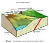
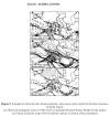
Seismic zoning is among the most complicated and extremely important problems of modern seismology. It is the foremost link in a complex chain of an estimation of seismic hazard and seismic risk. Seismic zoning is urgently needed for the total area of the Earth without a single exception, since large damaging earthquakes have occurred and can occur in the future, even in plains, which comparatively quiet, geologically speaking. Recent research has shown that about ten percent of Earth's surface is occupied by high or very high seismic hazard zones. These include all the countries situated along the Pacific rim, in the Mediterranean, the Near and Middle East, Central Asia, Himalayas, along the Trans-Asian belts and adjacent areas. About 70% of the land mass lies in a relatively low hazard zones. However, in such regions the seismic danger can be high also if low magnitude earthquakes occur at shallow depths because these territories are very densely populated.

Further fundamental and applied research in seismogeodynamics and seismic zoning is to focus on development of scientific principles and techniques to be used in dynamical seismic zoning based on studies in seismicity, migration of strain waves and seismicity increases, reoccurrence of earthquakes at the same location and other problems of earthquake generation that still remain unsolved. It is important to operate with extended earthquake sources, to use of the nonlinear recurrence graph and moment magnitudes, and to calculate a spectral shake-ability. Not less important is to study features of seismic effect depending on a type of geological structures generating the earthquakes (shear-fault, overthrust, normal fault, etc.).

1. Earthquake Hazard

Earthquakes are one of the most dangerous natural calamities influencing the human environment. They occur very frequently. Earthquakes begin very suddenly aggravating their destructive consequences. Often as destructive as the earthquake itself are the resulting secondary effects: surface faulting, tectonic deformation, landslides, tsunamis, floods, fires and blasts (Figure 1). Earthquakes and their numerous aftershocks affect the human psyche, cause serious cardiac-vascular, endocrine and other diseases. These problems as well as some new ones were encountered by medical and rescue units during the operations to mitigate the disastrous effects of strong earthquakes.

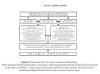
Figure 1. Earthquake source and its secondary effects

Unfortunately it is not yet possible now either to predict an earthquake and thus to avoid its consequences. However, their disastrous effects and the number of casualties can be reduced only by means of drawing up reliable maps of seismic zoning, by observing the standards of anti-seismic building and pursuing in seismic regions the long-term policy based on increasing the level of public awareness regarding the dangers involved, and the ability of the state and public services to withstand the natural calamity.

Earthquake hazard does not decrease with time, but actually increases in direct relation with the economical assimilation of seismically active territories and with the human influence on the Earth’s crust (uncontrollable pumping of oil and gas, extraction of other mineral deposits, the construction of major hydraulic structures, burial of industrial waste and the like). Enhanced seismic risk arises from nuclear power stations and other ecologically hazardous facilities installed in seismic regions, because even very insignificant earthquakes and secondary post-seismic consequences (rock slides, cracking in the ground etc.) can disrupt their normal operation.

Seismic zoning is a highly complex and extremely important challenge of modern seismology. This is to say nothing of the social, economical and ecological significance of this problem. Its scientific intricacy is based primarily on the fact that it belongs to that category of predictions based on incomplete information, on scant experimental data, not always derived from successful experiments, and on the methodological standpoints being insufficiently clear. Therefore, for example, in the United States, new seismic hazard maps are required by law every 5 years, in the Russia every 10−15 years. And although the maps of seismic zoning are being updated and improved periodically, as additional information on earthquakes becomes available and seismological knowledge is further perfected, these changes are fragmentary in that broad, universal data is not forthcoming from all corners of the globe, but is confined to those well-known, seismically active zones. Therefore, seismic zoning maps compiled in certain countries proved to be, to some extent , inconsistent with the actual natural conditions, which, together with low-quality civil engineering construction, caused many casualties and enormous material damage to the national economy.

Seismic hazard assessment is based on the observation and measurement of the ground shaking produced by seismic waves passing. The seismic effect depends on the magnitude of earthquake, the depth of its hypocenter, the distance from the earthquake source, the local ground conditions (e.g. rock or soft soil), etc.

There are two general approaches to seismic zoning: the historical records of earthquake occurrences (“Historic methods”) and the geodynamical interpretations of the seismicity and earthquake source zones (“Deductive methods”). The first official seismic zoning map for a code on aseismic building was published in 1937 in Russia and initiated regular compilation of such maps as the basis for regulating design and construction in civil engineering in seismoactive regions of this country. The research conducted in the 1950-1960s led to a new paradigm of seismic zoning. It was based on a two-step method of genetic seismic zoning and a deterministic-probabilistic assessment of earthquake hazard (S.V. Medvedev, I.E. Gubin, Yu.V. Riznichenko). According to this concept, the first, seismotectonic step involves identification of earthquake source zones, while the second, engineering step is concerned with the calculation of the seismic effect caused by these at the surface (Figure 2). This two-step model and the probabilistic approach to seismic hazard mapping have become widely accepted in world seismology in the late 1970s, especially after the well-known papers of American scientists (C.A. Cornell and others). In recent years the ideas of deterministic-probabilistic forecasting of dangerous seismic and other geological processes have begun to influence more and more actively into seismology and into the practice of building construction.

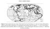
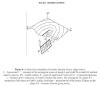
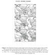
Figure 2. Structural chart of seismic zoning methodology.

Three database series (geodynamics, seismicity, and strong ground motion) are the basis used to develop two models: a source zones model and a model of seismic effects, which are used to calculate earthquake hazard and to map seismic zones.

Nevertheless, in spite of the high constructive value of this methodology, it is only the second, engineering, step of seismic zoning which has received much attention, i.e., calculation of seismic effect at the Earth's surface. The first step, identification and seismological parameterization of seismic source zones, which deals with deep-seated seismo-geodynamic processes and falls within the area of competence of seismologists and geophysicists, has remained less developed, being largely a subjective procedure. At the same time, already for a long time it became clear that since the zoning of earthquake hazard exclusively relies on the information concerning past earthquakes, without deep study of regional and global seismicity and without adequate earthquake source models, it is utterly hopeless. It became obvious that for seismic zoning of established local territories it is necessary to examine the features of geodynamics and seismicity in adjacent seismic regions that are genetically related to the area of interest.

There are a number of methods that have been used to estimate seismic hazard. However, these are not without their drawbacks. Here one of the methods is described, which is relatively more advanced, in comparison with others. The technique, described below, for identification of earthquake source zones and for calculating the seismic hazard is based on the seismic zoning ideas found within the approaches of Yu.V. Riznichenko in 1965, C.A. Cornell in 1968 and other scientists, but overcomes significant disadvantages of these approaches.

2. Global Seismicity

2.1. Global orderliness of seismogenic regions

The structural and geodynamic patterns observed in the extensive seismo-active regions of the Earth allow it to be treated as a global seismo-geodynamic system (SGD − system). These patterns are clearly expressed in the hierarchical heterogeneity of present-day tectonic features, ranging from the lithosphere to crust blocks of different ranks, as well as in the trends of their geodynamic evolution. The relation of regional seismicity to the structure and dynamics of the lithosphere is most clearly expressed on a global scale as three leading types of SGD-interaction caused by divergence, convergence, and transform displacements of the lithosphere plates.

The convergent lithospheric features are the most active seismically. They do not show an excessive scatter in size and are arcuate interplate boundaries extending along oceanic margins as subduction zones, as well as continental relicts of subduction zones (Figure 3). The dimensions of oceanic, hence continental, arcuate features are controlled by earth curvature, as well as by plate strength and thickness, and by the intensity of plate interaction. The mean length of all convergent regions worldwide is 3000±500 km. Roughly equal to that value are the dominant distances between the centers of two closest regions. The dimensions of these seismic regions and their spatial distribution have very direct bearing on the assessment of maximum possible earthquakes that can occur there.

Figure 3. Generalized tectonic map of the Earth showing boundaries (1 and 2) of major lithospheric plates and the global orderliness of earthquake-generating regional features: 1 - axes of convergent subduction zones and their relicts in continents; 2 - axes of divergent rift zones in oceans; 3 - direction of motion of plates.

Each region has its own seismic regime and seismicity structure; for this reason, as will be shown below, it is a region of the dimensions indicated above which is taken as the "basic" seismogenic structural unit to develop the model of earthquake source zones. The patterns that have emerged can become a basis for the appropriate seismic regionalization of the Earth.

Global seismicity is caused by the intense geodynamic interaction between several large lithosphere plates - the Eurasian, African, Arabian, Indian, North- and South-American, Antarctic and Pacific plates. Horizontal motion of the plates can be 10 centimeters and more per year.

Earthquake sources can occur in the region 0 - 700 kilometers below the Earth's surface. This earthquake source depth range is, as a rule, divided into three zones: shallow, intermediate, and deep. "Shallow" earthquakes are between 0 and 70 km deep, "intermediate" earthquakes, 70 - 300 km and "deep" earthquakes, 300 - 700 km deep. Earthquakes with depth up to about 700 km are localized within convergent subduction zones that are sinking into the Earth's mantle . The sources with intermediate depth occur mainly in relicts of such zones inside continents. Shallow are distributed practically everywhere. Most of the intra-crust earthquake sources are in the upper crust within 15 km of the ground surface. The vertical distribution of the hypocenters is controlled by the dimension L_M and vertical extent H_M of the relevant sources, which are related to magnitude M of the respective earthquakes.Annual occurrence of earthquakes on the Earth is as follows: one with Ì ≥ 8.0, about three with Ì ≥ 7.5, about 15 with Ì ≥ 7.0, about 60 with Ì ≥ 6.5, and more than 200 with Ì <6.5. Certainly, these mean that the yearly seismicity rate (V_M) is highly variable and longer period of observation could give quite different results.

2.2. Regional Structure of Seismicity

The seismic sources are not distributed chaotically. They arise in the most compliant inter-block contact zones and most often occur, in a regular manner, in fixed sites that are least favorable for creep displacements and thereby seismically most hazardous. Commonly, these seismogenic structures are intersections of faults or displacement zones, their sharp bends, or other features (asperities and barriers) that prevent slow tectonic movement on faults. If such delays are long, more elastic energy is collected; the large volume of rocks become potentially stressed and the next earthquake will be stronger. The dimension of such areas is determined by the sizes of interacting blocks bounded by active faults or displacement zones. These sizes control the upper threshold of the earthquake magnitude, and the number of blocks is responsible for the intensity of the tectonic movements and seismic regime (average number of seismic events per unit time). The fault ranks J, and the distances between their dislocated nodes δ_j, as well as block sizes are determined by the thickness and strength of the related layers faulted in the past geological epochs. The thicker the layer divided by faults into blocks, the larger and longer the faults and the greater the distances between them. This results in an increase in block sizes and, consequently, in the magnitude of the related earthquakes. Conversely, the number of faults, blocks and earthquake sources increase as the layer thickness decreases.

The lattice of the intra-continental faults is predominantly of the rectangular, or more often square shape determined by the tangential compression. It was found that the distances δ_j between the intersections of faults and, accordingly, the dimensions of geological blocks (geoblocks) exhibit a well-pronounced tendency of clustering in ranks, their vertical and horizontal dimensions being in a ratio of roughly two to one between adjacent ranks. This phenomenon seems to have its origin in the persistent doubling of the depths to major discontinuities in the crust and upper mantle, the faults of respective ranks penetrating as deep as the discontinuities. To take an example, the top of the "granite" layer in the continents lies at a mean depth of 10 km, the Conrad discontinuity is at 20-25 km, the crust-mantle interface is at 40-50 km, the bottom of the lithosphere at 100 km, that of the asthenosphere at 200 km, these being followed by the 400-km and 700-km discontinuities. This fundamental pattern of discontinuous change in material properties as the depth is multiplied by two governs all geological depths up to and even including the soil.

The orderliness thus emerging dictates a corresponding orderliness, not only in systems of tectonic faults and geoblocks, but also in the hierarchy of earthquake sources: the larger the earthquakes, the farther are their sources from one another. Thus, earthquake sources when ranked according to magnitude M and elastic energy radiated E are distributed in a regular manner, not only in time ("frequency-magnitude relation"), but also in space ("the law of inter-source distances"). It has turned out that the mean distances δ_M (km) between the epicenters of two closest-lying earthquake sources of length L_M (km) and magnitude M are well described by the following relations:

δ_M = 10^{(0.6
Ì - 1.94)} (1)

L_M = 10^{(0.6
Ì - 2.5)} (2)

As is apparent, the factor 0.6 at M implies that the source sizes L_M and distances between epicenters δ_M change approximately by a factor of two with a 0.5 increase in magnitude. From the above relations it follows that the quantity δ_M/L_Ì = 3.63 is independent of magnitude, thus reflecting self-similarity in the size hierarchy of geoblocks and the associated earthquake sources in the entire magnitude range investigated (from Ì = 6.0±0.2 to Ì = 8.0±0.2). Also independent of magnitude, to some degree at least, is the ratio of earthquake sources length L_M to the vertical sources plane extent H_M, which is identical with the respective thickness of the geoblocks.

Relations (1) and (2) are still neater when earthquake energy is expressed in the SI system, where E = 10^(1.8M+4) is measured in Joules, L_E and δ_Å in meters:

(3)

In that case δ_E/L_E = 3.5.

The quantity δ_M (as well as δ_E) is none other than the mean horizontal size δ_j of geoblocks that can generate earthquakes of the respective maximum magnitude M_max; δ_M= δ_j is the diameter of the area responsible for M_max, a very important quantity for the assessment of earthquake hazard; this is related to δ_j as follows:

M_max = 1.667 log δ_j + 3.233. (4)

Interrelationships in the orderliness of faults, geoblocks and earthquake sources, as well as in the evolution of seismogeodynamic processes are just more evidence in favor of a structural and dynamical unity of the hierarchical geophysical medium and the seismogeodynamic processes that are going on in it. Orderliness obtains also in the hierarchy of soliton-like strain waves (the so-called G waves, or geons) of seismicity increases. These provide for the dynamics of interacting geoblocks and for directivity in the evolution of synergistic seismogeodynamic processes. Geons propagate along faults of their respective ranks, creating and removing various barriers and so provoking earthquake sources of appropriate magnitudes. Since these geodynamic processes are evolving more or less independently at each hierarchical scale, they possess the same fractal dimension as for the fault-blocky medium and its seismic regime. When the external geodynamic excitations are low, the seismicity in the region is close to the steady state, involving small shallow earthquakes that are being generated by a denser network of smaller faults. When the external forces become greater, e.g., as a result of major coseismic or creep movements, the SGD-system passes to a qualitatively different and better organized state. Larger fault zones begin to "operate". This can be inferred from ordered changes in seismic activity in many regions worldwide (migration of earthquake sources, periodic seismic rate increases, localization of quiescent areas and the like) which are caused by synergetic self-organized phenomena typical of many hierarchical multi-component non-equilibrium systems.

3. Models of Earthquake Occurrence Source Zones

3.1. Lineament-Domain-Source Model

The identification of the zones of earthquake sources occurrence (zones of ESO) and the determination of seismicity parameters for them is the most complex and crucial part in seismic zoning work, because this determines the trustworthiness of all subsequent developments. According to the concept described above the basis for the model of ESO zones for seismic zoning is the Lineament-Domain-Source (LDS) model (Figure 4).

Figure 4. Major structural elements of LDS model for ESO zones.

Shown are plots of mean yearly seismicity rate V in the entire region (V_R) and in the constituent structural elements - lineaments (V_l), domains (V_d), and potential earthquake sources (V_s). The magnitude ranges proper to each type of feature also are shown

The LDS model contains four scales: a major region (R) with an integral seismicity characteristic and its three main structural elements, namely, lineaments (l_Μ), which roughly represent the axes of the tops of 3D earthquake-generating fault features and structured seismicity, and which form the backbone of the LDS model; domains (d_Μ), which cover the area without gaps and are characterized by diffuse seismicity; potential earthquake sources (s_Μ) indicating the most dangerous segments and which are generally confined to lineaments. The "driving force" in the LDS model comes from interaction between geoblocks and from the above mentioned geons which accommodate movements of block sides.

The structural ESO zone elements (lineaments, domains, and potential sources) are classified by maximum possible magnitude M_max, as are the earthquakes, at intervals of 0.5 magnitude units: M≤8.5±0.2, ≤8.0±0.2, ≤7.5±0.2, ≤7.0±0.2, ≤6.5±0.2 è 6.0±0.2. The sign "≤" indicates that each lineament with M_max also includes all smaller ones, down to M = 6.0 inclusive. The upper magnitude M_max is controlled by the relevant seismo-geodynamic environment, while the lower M_min is determined by completeness of reporting for earthquakes with the lowest magnitude that still poses some seismic hazard (usually M_min = 4.0 and the lowest intensity of shaking being I_min= V).

The magnitude M_max is assessed by all accessible and reasonable techniques: from the dimensions (δ_j, km) of interacting geoblocks, the width of zones of dynamical influence emanating from major seismogenic features, the length and segmentation of earthquake-generating faults, from archeological and historical evidence, the configuration of the frequency-magnitude relation, the extreme values in the plot of strain buildup in seismogenic features, the positions of potential earthquake sources likely to produce the maximum magnitude, and also from the dimensions of palae-seismodislocations (L_sd, km) according to the following relation:

Mmax = 1.667 log Lsd + 4.167. (5)

In order to identify the structures generating seismic waves and to estimate their seismic potential, it is important to use the mapping of the sources of earthquakes with various magnitudes in accordance with their size and orientation rather than the mapping of abstract "point" epicenters as is commonly done. The size and orientation of source are determined from the distribution of aftershocks, coseismic ruptures, maximum isoseismic lines, focal mechanisms, geodetic measurements, analysis of tectonic events, and so on. In accordance with the new map legend, sources of earthquakes with M ≥ 7.0 (M ≥ 6.8) are shown as ellipsoids in "natural" sizes. The large L and small W axes of the ellipsoids, as well the conventional diameters L' of spheres for weaker sources, are calculated by the formulas conjugated at the level M = 6.5:

Ì≥6,5: logL = 0,6M - 2,5; logW = 0,15M + 0,42; logL/W = 0,45M - 2,92;

Ì≤6,5: logL`= 0,24M - 0,16. (6)

Seismolineaments serve as the main carcass for the LDS model of ESO zones and represent in a generalized form the axes of the upper edges of the three-dimensional and relatively clearly defined (concentrated) seismo-active structures at the Earth's surface. They trace the geoblock boundaries, which are characterized by the most contrast tectonic activity. Lineaments are identified by cluster analysis of the space-time distribution of "chains" of earthquake sources of corresponding magnitudes, as well as from the geophysical fields (especially from their gradients), from palae-seismodislocations, cosmic photographs, from the similar historic-tectonic development in the Cenozoic era (predominantly in the upper Pleistocene and Holocene), from activity in the Quaternary period, from the close values of velocity gradients of neotectonic movements and from other signs of recent and modern geodynamics. Lineaments and their segments are characterized by the magnitude of the maximum possible, within their limits, earthquake M_max ; by their length l_iand width w_i due both to their tectonic nature and the errors in determining their dislocation; by the depth of bedding of the upper, h_min, and lower, h_max, edges of the plane of seismogenic structure; by the strike azimuth Az⁰; by the dip angle a⁰; by the type of predominant displacements (shear-fault, overthrust, normal fault and so on). Lineaments can exhibit strikes of most diverse types due to the tectonics of a region and can intersect each other, which "automatically" increases the seismic hazard in their dislocated nodes in calculations owing to seismic effects from the summing up of nearby located sources.

Domains (d_Μ) are volumetric areas less pronounced as far as structure is concerned or inadequately studied seismogenic zones characterized by "quasi-homogeneous" tectonics and relatively weak seismicity. They embrace layers of thickness from h_min to h_max kms. Unlike lineaments, domains do not intersect each other, and they cover all the investigated territory without breaks and superposition. An apparent intersection is characteristic of domains belonging to different depth layers, i.e. in the subduction zones and their relict on the continents: Himalayas (especial their northwest and southeast endings), Hindu Kush, Eastern Carpathians, Caucasus and in other regions. As it has been mentioned, the "domain" concepts (as well as the concept of "quasi-homogeneous" seismo-tectonic provinces) is the cost related to difficulties, associated with revealing the more fine structure of focal seismicity from weak earthquakes, due to errors in determining the locations of their epicenters. Actually, there is no doubt that focal seismicity is structured at all scale levels.

Potential Sources (s_Μ) of earthquakes identified by various methods (from dislocations, from the dominant distances between epicenters, by methods of pattern recognition, and so on) are, as a rule, confined to seismolineaments, and their dimensions L_s are related to the magnitude of the maximum possible earthquakes. Potential sources have the same parameters as the respective lineaments (shear-fault, normal fault, overthrust, and so on).

Generalized seismic zoning (GSZ, maps to scale 1 000 000 and less) will identify with some confidence lineaments that generate earthquakes of M ≥ 6.0. This magnitude threshold can be lowered for areas covered by detailed seismic zoning (DSZ, maps of 500 000 and large scale).
According to the LDS model, as was pointed out above, each lineament that can generate earthquakes of M_max also includes lineaments of smaller ranks, down to M = 6.0 inclusive, because these also produce (with some deviations across the feature) earthquakes of lower magnitudes as well. Events of M_max≤5.5 generally belong to domains. Potential earthquake sources have definite magnitudes (usually M_max≥7.0) and most frequently occur on lineaments.

Since the actual earthquake sources do not occur strictly along lineament axes, but deviate from these in some way, it is possible to calculate the mean deviations. The lower the magnitude, the farther the sources may stray from the relevant lineament axis. It is useful for bringing the model closer to what is actually observed in nature. According to the LDS model, the top of the associated sources reach (but do not go beyond) the top of the consolidated crust, although the earthquake sources themselves and the associated hypocenters involve a greater scatter in depth of focus, since the depth distribution of larger earthquakes is controlled by the vertical extent of the source planes. In addition to nearly vertical sources planes (90⁰±20⁰) usual on strike slip faults, lineaments are characterized also by two different ranges of dip, 45⁰±20⁰and 135⁰±20⁰for thrusts and for normal faults. The resulting characteristics of seismicity behavior and the scatter of earthquake sources are further used in subsequent work to model a predicted (virtual) seismicity, to calculate repeat times of intensity in seismic zoning.

Disregarding for the moment the type of geodynamical fault movement (strike slip, thrust, normal faulting, etc.), it is possible to assume that in a first approximation all faults of one and the same rank in a region, accommodate the geodynamical stress and strain built up there, on an "equitable" basis. This justifies the procedure whereby seismological parameterization of the ESO zones has the rate of seismic events with respective magnitudes distributed in direct proportion to lineaments length.

3.2. Seismic Regime of Earthquake Source Zones

The basic quantity in calculating seismicity parameters for the main structural ESO elements is the total rate of seismic events per unit time (one year here) V_RM in a specified region (see Figure 4). A regional rate V_RM is found from the relevant earthquake catalog with aftershocks, foreshocks and other clustered events eliminated, and taking into account the recording periods for respective seismic events. For each specified magnitude range ΔÌ=±0.2 one finds the mean long-term rate of events V_R corresponding to their mean number N_RM or the mean yearly probability P_RM(1) that at least one earthquake with this magnitude will occur in the entire region R.

All plots of log V(M) are evidently nonlinear (see Figure 4). It is only for the magnitude range 4.0 ≤ M ≤ 6.0 that one finds straight parts with slopes close to b = −0.9. In the range M ≥ 6.5, however, all plots without a single exception develop an upward bend, indicating a higher rate of occurrence for these events than would follow from a conventional linear (that is exponential) extrapolation of the left parts to the right. The actual rate of occurrence for larger earthquakes is higher by a factor of three or more than what it was previously believed to be. The use of straight plots so far significantly overestimated the return periods of larger events, hence underestimated seismic hazard in many seismically active regions.

Since the seismic regime of any structural ESO element (l_M, d_M, s_M) is controlled by the total rate in the region (V_RM), the plots of V_l, V_d, V_s in each element will have configurations similar to the relevant regional plot shown in Figure 4 and be absolutely identical with it when summed over all elements ("the law of conservation of seismic energy"):

ΣV_lì+ΣV_dì+ΣV_sì =V_RM. (7)

Seismological parameterization of each lineament (and of segments of lineaments as well) requires the total length (Σl_Ì) to be calculated for each region; this consists of the lengths _Σl_Ì of all lineaments of this and higher ranks, since, as mentioned above, lineaments with M_max also include all those with M<M_max down to and including M = 6.0. The next step is to find the mean yearly rate V_lM for the events of the relevant magnitude along each lineament (and segments of these) l_M in length as being part of V_RM, which is the total rate of seismic events with this magnitude in the region:

V_lì = V_RM l_Ì / Σl_Ì. (8)

The rate of seismic events in a domain, V_dM, is simpler to find; this is based on a selection from the standardized catalog of all M≤5.5 events occurring in the domain of interest and plotting the associated frequency-magnitude relation. It goes without saying that the law of conservation of seismic energy must hold in this case too, because the rate of events in a domain is also part of the total rate (V_RM) in the region for the magnitude range 4.0≤M≤5.5. Expert assessment is at present used for aseismic or low seismicity regions.

The rate V_sM at potential M_max sources is defined as the part of V_lM on the relevant lineaments, but the earthquakes taken into account here are only those with this particular magnitude M = M_max rather than the total rate with M<M_max as is the case for ordinary lineaments, i.e., excluding the regular background seismicity for the relevant lineament segment and the aftershocks of the potential sources.

The distribution of lineaments with different ranks over M_max for regions is an overall reflection of the fractal dimension U~ −0.9 for the entire hierarchical set of lineaments, which is consistent with the most popular mean b-value (b~ −0.9). Indeed, both sets of curves (b-value and U-value) for the magnitude range Ì ≥ 6.0 have similar configurations as well, thus corroborating the idea of nonlinear frequency-magnitude relations and of a structural-dynamical unity of the geophysical medium and the seismic processes going on in it, hence that the LDS model is realistic.

It should be noted that the identification and adequate seismological parameterization of lineament structures play the important role for reliable estimation of seismic hazard. The representation of seismogenic structures only as "quasi-homogeneous seismo-tectonic provinces" (domains in this terminology) with their scattered seismicity, which has been widely accepted until recently, is less realistic from both the seismological and geotectonic standpoints. Although the scattered seismicity does not actually exist in nature, seismologists are compelled to use such an approach, as well as the domain ("seismo-tectonic province") model, because knowledge of the fine structure of the seismic medium is incomplete. In this respect, the most rational way is to construct a hybrid lineament-domain model which is presented in this paper. However, the overall replacement of high-amplitude lineaments by spatial domains is unacceptable for physical reasons. Moreover, this is unjustified for the following two reasons. First, a decrease in the domain area without regard to the size of zones responsible for large earthquakes increases the recurrence period of such events and, consequently, underestimates the seismic risk, resulting in errors of the "missing target" type in seismic zoning maps. Second, an excessive enlargement of the domains within which high-magnitude earthquakes are possible makes the seismic risk pattern more diffuse and gives rise to errors of the "false alarm" type.

The lineament-domain-source model of ESO zones, based on the probabilistic-determinate fractal lattice regularization of the parameters of regional seismicity and recent geodynamics avoids these shortcomings and adequately incorporates the specific features of the distribution of earthquake sources for various magnitudes. Another innovation is the practical use of extended, rather than "dot", seismic sources, adequate to the real natural conditions (size, azimuth, etc.) in the seismic risk assessment and mapping.

The new method of creation of the ESO zone models and their application to the seismic zoning was named "Earthquake Adequate Source Technology - EAST-97".

3.2. Virtual Seismicity

Figure 5 illustrates an example of the sequence of creation of LDS model and virtual seismicity map for the Iran-Caucasus-Anatolia region. Figure 5 a shows the observed earthquake sources of different magnitudes and sizes L_M: M≥8.0±0.2 (large ellipses L = 200 km long); M=7.5±0.2 (medium ellipses 100 km long); M=7.0±0.2 (small ellipses, 50 km); M=6.5±0.2 to M=5.0±0.2 at intervals of 0.5 magnitude units (circles of decreasing diameter).

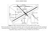
Figure 5. Example of observed and virtual seismicity, and source zones model for the Iran-Caucasus-Anatolia region: (a) Observed earthquake sources of M≥5.0; (b) Lineament-Domain-Source Model for the region; (c) Virtual seismicity map of M≥5.0 and the scheme of seismic effect calculation.

On the basis of regional seismicity, seismo-tectonic and seismo-geodynamic of this test area . LDS model shown on a Figure 5 (b) is created. Here are shown: l - seismogenic lineaments with M_max= 8.0 ± 0.2; 7.5 ± 0.2; 7.0 ± 0.2; 6.5 ± 0.2; 6.0 ± 0.2 (line thickness decreasing by a factor of two for the respective magnitudes); d -domains having different M_max≤5.5; s - potential sources with size L_s corresponding L_M.

Figure 5 (c) shows an example of predicted seismicity for the Iran-Caucasus-Anatolia region obtained by computer generation of virtual earthquake sources based on a long-term synthetic catalog generated in accordance with the LDS model for ESO in this region and with their mean long-term seismic regime. The virtual seismicity map shows the synthesized sources as the projections of the horizontally extended rectangles onto the Earth's surface. The rectangle size is related to the magnitude of possible earthquakes (in the given case, M≥5.0). The width of the rectangles depends on the fault plane dip angle (see Figure 6). The map shows an example consisting of a random sample for a 100-year time interval. To take into consideration the great number of statistically dependent factors, the technique is applied for Monte-Carlo calculations based on the extended in time random catalogue of earthquakes. The usual number of samples is 20-30, while the time interval is specified depending on the assigned probability of exceeding (or non-exceeding) for expected earthquake hazard (see below).

Figure 5 (a) shows the observed seismicity of the region for purposes of comparison. The two maps (Figures 5 a and 5 c) look similar, demonstrating that the LDS model of ESO is realistic.

The calculation of strong ground motion is carried out for each node of grid with size 10 × 10 km² (or other, depending on scale of a map and desirable detail) covering the region and adjacent area. For each node of grid ("receivers") a histogram of intensity occurrence is made, these data being the basis for subsequent mapping of earthquake hazard and related tasks (see Figure 5 c).

4. Model of Seismic Effect

The final phase of seismic hazard assessment involves calculation of seismic effects at the earth's surface due to each individual virtual source taking into account its dimensions and the attenuation law of seismic ground motion. The attenuation of ground shaking is, as a function of earthquake size and distance, taking into account propagation effects in different tectonic and structural environments and using direct measures of the damage caused by the earthquake and instrumental values of ground motions.

The model takes into account "saturation" effects of the intensity near the source, the nonlinearly of the intensity-distance relationship I(log r) and "saturation" of the magnitude for large seismic moment M₀, i.e. the problem of overstating the intensity for small distances and the isoseismic ellipticity is modeled automatically within the near zone for the sources of large magnitudes.

As was mentioned above, the calculation of seismic hazard is based on simulation of the earthquake catalogue. The intensity-magnitude-distance relationship I(M, r) is modeled from the regional empirical data. To approximate these data and to predict the intensity, the model of such a relationship is used that assumes the idea of an incoherent extended source in the form of a radiating rectangle with its long side parallel to the Earth's surface (Figure 6).

Figure 6. A scheme for calculation of seismic intensity from a single source. C - hypocenter, C` - epicenter of the rectangular source of length L and width W on depth H, inclined under a corner j; XY - Earth's surface, P - point of supervision ("receiver"), r - hypocentral distance, r_i - distance up to i-subsource, on which is broken the source. The rectangular on a plane XY - projection of the source to Earth's surface, bold edge - projection top of the source. Ellipses on the plane XY - isoseists from the given source. The intensity I of shaking at the nodes of the grid covering the region under investigation is calculated for each event of the model catalogue from the intensity-magnitude-distance relationship applying formula (9):

(9)

where I_B- intensity from "basic" source with magnitude M_wB on the distance r_B; C_M - coefficient connecting I and M_W; C_A - coefficient connecting I and maximum acceleration A of ground shaking, and duration d₅₀ of the part of the accelerogram with amplitudes exceeding 50% of the maximum; r - distance from the centre of a rectangular source involving N elementary emitters; Φ(r_i) is the attenuation function of damping, r_i is the distance from the elementary radiator to the receiver.

5. Probabilistic Seismic Zoning

As a basis for the seismic zoning map, the map is adopted for the calculated intensity I with a fixed return period T at each point on the map (once every T years on the average). This I value is denoted as I_T. The recurrence of intensity I events is the mean yearly number of earthquakes causing shaking of intensity ≥ I. A recurrence of once in T years, on the average, means that the probability of exceeding the intensity I_T during t years (i.e. that at least one such an event will occur) is equal to P = 1 − exp (−t/T), and P = t/T when t << T. For example, P is approximately 10% (the precise value is 9.52) for T = 500 years and t = 50 years; P ~ 5% (the precise value is 4.88) when T = 1000 years and t = 50 years.

The map of the calculated intensity I_T (the seismic hazard map) is calculated from the long-range characteristics of seismicity in a region with the use of the regional dependence of intensity on magnitude and distance for an extended source. From the values of I_T at the nodes of the grid obtained in a described way, the map of seismic hazard (represented by I_T value) is prepared.

The set of seismic zoning maps shown in the Figure 7 is based on the recent advances in the field of seismology and seismic zoning. The maps of intensity recurrence I were developed, as pointed out above, using a synthetic earthquake catalog generated from a model of predicted seismicity (LDS model for ESO) incorporating the attenuation of ground motion with distance.

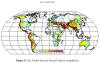
Figure 7. The fragment of seismic zoning maps for Iran-Caucasus-Anatolia region which in 1993 -1995 was test area of the Global Seismic Hazard Assessment Program (GSHAP, look below). The probability of a specified intensity at any point of a zone to exceed during 50 years is (%): a − 10; b − 5; c − 1, corresponding to mean period T = a-500, b-1000, and c-5000 years repeat times for these intensities for medium soil.

These maps can be used to assess earthquake hazard for structures with differing time life and degrees of importance at three levels to show theoretical intensity of earthquake shaking I to be expected in a given area at a given probability P during a given interval of time t (t = 50 years in the present case):

· the (a) map is for 10% probability of exceeding (or 90% probability of non-exceeding) for a design intensity during 50 years, with frequency of once every T = 500 years (the precise value is 475 years);

· the (b) map is for 5% probability of exceeding (or 95% probability of non-exceeding) for a design intensity during 50 years (T = 1000 years; the precise value is 975);

· the (c) map is for 1% probability of exceeding (or 99% probability of non-exceeding) for a design intensity during 50 years (T = 5000 years; the precise value is 4975).

Under a different interpretation, (a), (b) and (c) maps characterize 90% probability of non-exceeding (or 10% probability of exceeding) for a design intensity during approximately 50, 100, and 500 years, respectively.

Certainly the choice of a degree of acceptable risk is really an economic or political decision, not seismological one.

6. Global Seismic Hazard

The global seismic hazard map (Figure 8) was assembled by the U.S. Geological Survey and the Swiss Seismological Service in 1999 under general leadership of Prof. D. Giardini, general coordinator of the Global Seismic Hazard Assessment Program (GSHAP). This map is a product of the GSHAP, launched in 1992 as a demonstration project of the United Nations International Decade of Natural Disaster Reduction (UN/IDNDR), conducted by the International Lithosphere Program with the goal of improving global standards in seismic hazard assessment. Hundreds of scientists from most of the world's countries cooperated to produce the map. The GSH map depicts the global seismic hazard as peak ground acceleration (PGA) with a 10% chance of exceeding (90% chance of non-exceeding) in 50 years, corresponding to a return period of 475 years. PGA can be applied to building codes.

Figure 8. The Global Seismic Hazard Map (simplified).

The GSH map, which took seven years to complete, incorporates a number of existing country maps. It includes data from seismic networks, instrumental catalogs from different regions, historical and recent seismicity, palae-seismology studies, geodetic monitoring, and geologic and tectonic framework studies. The GSH map has been compiled by joining the regional maps produced for different GSHAP regions and test areas including Iran−Caucasus−Anatolia region, shown above in Figures 5 and 7. This Caucasus research project supported by INTAS for countries of CIS (Russia, Armenia, Georgia, Azerbaijan, Ukraine, Turkmenistan) and Europeans countries (Italy, Switzerland, Germany) was established as an international test area for seismic hazard assessment in the Caucasus, in co-operation with the International Association of Seismology and Physics of the Earth's Interior, the European Seismological Commission, the UN/IDNDR Global Seismic Hazard Assessment Program, and with organizations in neighboring countries (Iran, Turkey). This project as well as GSHAP focused on networking teams of specialists already active in the main elements of seismic hazard assessment: earthquake catalogues and databases, seismotectonic and earthquake source zones, and strong seismic motion of the ground. Computation of seismic hazard was performed by testing and comparing of different approaches, such as historical probability, seismo-tectonic probability, and real probabilistic assessment.

The map measures peak ground acceleration (m s^-2) and provides seismic values for grid of about 10×10 kilometers in every direction. The map colors chosen to delineate the hazard roughly correspond to the actual level of the hazard. The cooler colors represent lower hazard while the warmer colors represent higher hazard. The largest seismic hazard values in the world occur in areas of the largest lithosphere plate boundaries and their relicts on the continents. Despite the small percentage of land located in high hazard zones, many of the world's megacities lie within these zones. The red and brown swaths cover a number of areas, including plate boundary regions along the Pacific rim, the Mediterranean, the Near and Average East, Central Asia, Himalayan and Trans-Asian belt.

Until present time, peak ground acceleration has been used as the most popular parameter for the earthquake hazard assessment. However, it doesn't always correlate well with the actual character of damages because the degree of damage of different buildings depends not only on the value of acceleration but also on the spectrum of seismic waves. Thus, maps of seismic zoning should characterize not only a simply PGA value, but also a spectral of seismic shaking. Therefore it is recommended that the hazard should be calculated separately for a range of frequencies, using the same source zone model, and an adequate model of regional spectral attenuation for seismic effect. But it is now very difficult since strong ground motion recording instruments are still not widely used in seismological practice.

Fixation of the huge file of initial and target data in a digital electronic form within the Geographical Information System (ESRI GIS) is a distinct fundamental achievement of the new technology of seismic zoning as compared with all previous technologies. It permits obtaining rapidly reference analytical information on all the parameters and to use the SHA materials for the preparation of maps of larger scales on their basis, as well as to estimating the seismic hazard, the seismic risk and vulnerability of specific regions and countries. In case some additional data is revealed on seismic hazard (the discovery of hitherto unknown palae-seimodislocations, of new historic information on past earthquakes, of the migration of seismic activation, and so on) the database allows to rapidly incorporate any necessary corrections into the calculations of seismic hazard and, correspondingly, into its mapping.

Acknowledgements

The author is grateful to Prof. Dr. Domenico Giardini, Swiss Seismological Service Director, coordinator for the Global Seismic Hazard Assessment Program (GSHAP), Prof. Dr. Alexander Gusev and Dr. Lidia Shumilina compiled the seismic hazard algorithms and software for the new methodology, and to all numerous scientists who have taken part in GSHAP for Northern Eurasia.

Related Chapters

Glossary

Earthquake	: Shaking of the Earth surface caused by a sudden movement of rock beneath its surface.
Aftershocks	: Shocks which generally follow a larger earthquake (a main shock) and originates in or near the rupture zone of the larger earthquake. Sometimes, the main shock is preceded by foreshocks. Sometimes, earthquakes occur in sequences which are called doublets, triplets, multiplets, or swarms depending on how many similar-size events are in the sequence.
Fault	: A fracture or fracture zone in the Earth's crust or in upper mantle along which displacement of two sides relative to one another has occurred parallel to the fracture. A fault is active if it can undergo movement from time to time in the immediate geologic future.
Hypocenter	: The location of the point (or focus) within an earthquake source from which the rupture of rock and first elastic waves originate. A point on the Earth's surface directly above the hypocenter of an earthquake is called an epicenter.
Intensity	: (I). A numerical index (generally from I to XII) describing effects of an earthquake on the Earth's surface, on humans, structures and/or the land itself. The intensity at the point depends not only on a strength of the earthquake (magnitude) but also on a distance from the earthquake to the point, spectral characteristics, and the local geology at that point. Structural engineers usually contribute information for assigning intensity VII or above.
Magnitude	: (M). A quantity characteristic of strength of an earthquake or strain energy released by it determined at seismic stations. This is a logarithmic value originally defined by Charles Richter (1935). There are several different magnitude scales including: local magnitude (M_L), surface wave magnitude (M_S), and body-wave magnitude (m_b), moment magnitude (M_W). The scale is theoretically open ended, but the largest known earthquake have had M_S magnitudes 8.9.
Peak Ground Acceleration	: (PGA). The maximum value of ground motion acceleration as it is displayed on an accelerogram. At the strongest earthquakes the PGA can exceed the value of acceleration of gravity.
Seismic Domain	: An area of homogeneous or nearly homogeneous seismo-tectonics with mainly general orientation of a series of active faults distinguished by the structure, geodynamics, seismic regime and spatial distribution of earthquake sources with different magnitudes.
Seismic Hazard	: A probability of occurrence of ground shaking in a given time period associated with the recurrence of earthquakes. The assessment of seismic hazard is the first step in the evaluation of seismic risk.
Seismic Lineament	: A rectilinear or nearly rectilinear narrow zone (axis) of earthquake sources distribution reflecting the extended seismogenic faults of the Earth's crust and lithosphere, characterized by specific geodynamics, seismic regime and maximal magnitude of earthquakes.
Seismic Risk	: A social-economic assessment obtained by combining the seismic hazard with vulnerability factors (type of buildings and infrastructures, population density, land use, date and time of the day, etc.).

Bibliography

Giardini D. and Basham P. (1993). The Global Seismic Hazard Assessment Program (GSHAP). Annali di Geofisica, Vol. XXXVI, N 3-4, June-July, Special issue: Technical Planning Volume of the ILP's "Global Seismic Hazard Assessment Program" for the UN/IDNDR, 257 pp. [Presents the Proceeding of the GSHAP Technical Planning Meeting, Rome, June 1-3, 1992.]

Gubin I.E. (1950). Seismo-tectonic method of seismic zoning, Trans. Geophys. Institute, Moscow: AS USSR, N 13 (140), 60 pp. (in Russian) [Informs about new seismotectonic (“seismogenetic”) method of earthquake source zones identification for general seismic zoning]

Gusev A.A., Shumilina L.S. (1995). Certain aspects of the technique of general seismic zoning. Seismicity and seismic zoning of North Eurasia (edit. V.I. Ulomov), Issues 2−3, Moscow, UIPE RAS, p. 289-300. [Informs about new technique of seismic danger calculation for general seismic zoning]

Cornell C.A. (1968). Engineering seismic risk analysis, Bull. Seis. Soc. Amer., 58, p. 1583-1906. [The most famous publication which has begun world researches of seismic hazard assessment.]

Medvedev S.V. (1947). To a question on the account of seismic activity of area with construction, Proc. of the Seismological Institute, AN SSSR, N 119 (in Russian). [Presents the first, but not well-known in the world, publication about a probabilistic seismic hazard assessment.]

Riznichenko Yu.V. (1965). From the activity of seismic sources to the intensity recurrence at the ground surface, Izv. AN SSSR, Fizika Zemli, 11, p. 1-12 (in Russian). [The most developed methodology of a probabilistic seismic hazard assessment and calculation of spectral "shake-ability".]

The Global Seismic Hazard Assessment Program (GSHAP) 1992-1999. Summary Volume. (1999). Annali di Geofisica, 42, N 6, December, 1230 pp. [This work edited by Domenico Giardini presents the first-ever quantitative Global Seismic Hazard Map, provides updated seismic hazard values for nearly half of the world's nations.]

The practice of earthquake hazard assessment. (1993). International Association of Seismology and Physics of the Earth's Interior and European Seismological Commission. 284 pp. [This work edited by R.K. McGuire presents fifty-nine reports covering 88 countries, which comprise about 80 percent of the inhabited land mass of the Earth.]

Ulomov V.I. (1999). Seismo-geodynamics and Seismic Zoning of North Eurasia. Vulcanology and Seismology. N 4−5. p. 6−22 [in Russian]. [Presents the new methodology of seismic hazard assessment.]

Ulomov V. and Working group. (1999). Seismic hazard of Northern Eurasia. Annali di Geofisica, 42, N 6, 1023−1038. [Presents the new methodology and seismic hazard map for N 7 GSHAP region of Northern Eurasia in PGA value.]

Biographical Sketch

Valentin I. Ulomov was born in 1933, in Tashkent, Uzbekistan Republic. He is Professor of geophysics, Doctor of physics and mathematics, and Member of the Uzbekistan Academy of Sciences. His scientific interests are as follows: deep structure of the lithosphere; processes in earthquake sources; regional and global seismicity; seismo-geodynamics; seismic zoning; earthquake prediction. In 1955 V.I. Ulomov received the specialty of a mining engineer-geophysicist and was invited to work as a scientific researcher at the seismic station of “Tashkent”. In 1959 he became the head of this station. In 1963 he was the Deputy Director of the Institute of Geology and Geophysics, Uzbekistan AS, and the Director of the Tashkent Seismology Observatory. In 1966, he initiated creation of the National Institute of Seismology and became its Deputy Director. In 1966 V.I. Ulomov headed the complex studies of the Tashkent earthquake, whose source was located beneath the central part of the Uzbekistan capital. His scientific paper from 1967 about the prognostic properties of radon emission became widely known, and the radon method of searching earthquake precursors was quickly propagated all over the world. On the basis of many-years seismologic and strain observations, V.I. Ulomov officially predicted (in scientific publications of 1966-1974) the strongest Gazli earthquakes of 1976, on the Turan plate. In 1990 V.I. Ulomov moved from Tashkent to Moscow on invitation of the Institute of Physics of the Earth, where he became the head of the Laboratory of Continental Seismology created by him. From 1990 to 1997 V.I. Ulomov headed the studies on general seismic zoning of the territory of the former USSR and adjacent regions; in 1992-1999 he was one of the main participants of the Global Seismic Hazard Assessment Program (GSHAP). V.I. Ulomov is the author of more 300 publications.

To cite this chapter:

V.I. Ulomov, SEISMIC ZONING, in Natural Disasters, from Encyclopedia of Life Support Systems (EOLSS),

Developed under the Auspices of the UNESCO, Eolss Publishers, Oxford ,UK, [http://www.eolss.net]

©UNESCO-EOLSS

Encyclopedia of Life Support Systems